|
|
|
The plt pseudo object can be thought of as a super axis and in that respect it's
similar to Matlab's plot and plotyy functions but as you will learn it is much more than that.
It may be confusing at first that plt is both the name of a pseudo object as well
as the name of the whole toolbox. In fact all the pseudo objects describe here are
created, modified, and queried by using calls to the same plt()
function. The plt pseudo object differs from the remaining pseudo objects in that:
- For the remaining pseudo objects, the first plt argument will always be the name of
the pseudo object (as a string) but this is not true for the plt pseudo object.
To create a plt pseudo object, one or more numeric arrays are always required to specify
the points to be plotted and usually we put these arrays at the beginning of
the argument list which makes it more obvious that we are creating a plt pseudo object.
It is not strictly necessary to put the numeric arrays first and a call to plt will
still create a plt pseudo object when the first argument is a string, as long as that
string is not one of the following 21 strings (not case sensitive):
| click | dateStr | help | metricp | rename | version
| | close | edit | helpText | misc | select
| | colorPick | grid | hideCur | move | show
| | cursor | hcpy | markEdit | pop | slider
|
- When a plt pseudo object is created, two other pseudo objects are automatically
created as well (namely cursor and grid)
- A new figure window is immediately created to contain the plt pseudo object.
- The plt pseudo object may be called from the command line (similar to Matlab's
plot command) whereas it only makes sense to use
the other pseudo objects inside a .m file.
- Nearly every other section of this help file is dedicated to describing the details of the plt pseudo object.
|
|
cursor(pseudo
cursor
object)
|
|
The cursor pseudo object, more than any of the others is what gives the plt toolbox such
an advantage for GUIs involving plotting and data exploration. Once you get used
to the smooth and natural methods provided for cursoring, zooming and panning you will wonder
how you lived without them and you will want all your GUI tools to be similarly equipped.
The description of the cursor pseudo object is long to fit comfortably in this table, so a
separate section of the help file (which you will find here)
is dedicated for that purpose. That section describes how to query and modify the cursor objects
as well as how to create a cursor object using the 'init' action.
(It's not likely worth your time to review the 'init' action details because normally you will
let the plt pseudo object create the cursor object for you.)
|
|
grid(pseudo
grid line
object)
|
|
The trace color of the native Matlab axis grid
lines can't be independently set leading to grid lines that over power the
display. The grid line pseudo object is designed to solve this problem by
providing grid lines of whatever color and style you choose.
Actually the grid line problem I referred to is mostly solved in the latest R2014b
version of Matlab, however you can't use that capability if you need to remain
compatible with older Matlab versions. plt doesn't have this problem and the grid
lines will look wonderful on all supported Matlab versions (ver 6.1 thru R2014b).
Grid lines are positioned at each tick label. Additional (sub-decade) grid lines will also
be used for logarithmically scaled axes that span six or fewer decades. (The
six decade limit may be changed by adjusting the logTR
figure application data property which defaults to 1.0e6)
The grid line functions are:
plt('grid',ax,'init',color,erMode,LineStyle,In7,In8,In9,In10)
- Initializes grid lines on axis
ax of color color
with erase mode erMode
and LineStyle LineStyle.
- color is optional with default [.13 .13 .13]
- erMode is optional with default 'xor'.
- LineStyle is optional with default '-'
- In7,In8 is an optional parameter/value pair to apply to the grid lines
- In9,In10 is an optional parameter/value pair to apply to the grid lines
The pltvbar.m demo program uses this call to create a tabular
list next to the main plot area. Although that demo as well as the
three line example below calls this 'init' action, you will rarely
if ever do this because the grid pseudo object created automatically
by the plt pseudo object is usually sufficient.
plt('grid',ax,'toggle') - toggle grids (on/off)
plt('grid',ax,'get') - get grid line handle
plt('grid',ax,'off') - turn grids off
plt('grid',ax,'on') - turn grids on
plt('grid',ax,'update') - update grids
plt('grid',ax) - same as above
plt('grid') -
equivalent to plt('grid',gca)
All the above calls return the grid line handle. Setting ax to zero
in any of these commands is equivalent to specifying gca.
To experiment with these functions, try typing this at the command prompt:
>> plt('grid',axes,'init',[.7 1 1]); % create axis & grid pseudo object
>> set(gca,'ylim',[0 6]); % change axis limits
>> plt('grid'); % update grid lines
|
|
|
|
The slider control is Matlab's most versatile ways to control a numeric parameter because it
allows us to change a value continuously and repeatedly using several different methods
(click & hold on an arrow, click & hold in the trough, and dragging the slider bar). The pseudo
slider object (described later in this table) enhances this capability further by providing more movement
options and coupling it with the labels and numeric readout normally needed with the slider.
The only downside to the pseudo slider is that it takes up too much space to use it everywhere in a
GUI containing many numeric controls. For this reason an edit box
(i.e. uicontrol('Style','Edit')) is often used to control a numeric parameter.
However because the only way to change the value of an edit box is to type in a new number, it is
difficult to use when many adjustments are needed to arrive at an optimal setting or when you want
to develop a feel for the effect of small changes in the parameter. The edit
pseudo object was designed primarily to overcome that difficulty, although it also has the following
additional advantages over the uicontrol edit box:
- A label is almost always required for a numeric parameter and is sometimes needed for string
parameters as well. The uicontrol edit box doesn't have this label so you must add another
uicontrol for that purpose, complicating your program and making it more difficult to reposition.
The edit pseudo object includes an optional label so when you move the edit object its label
automatically moves along with it.
- The edit pseudo object may be positioned using figure coordinates or using the normalized or
data coordinates of an axis. Which coordinates to use is usually obvious and depends on the
use of the particular control. (The uicontrol edit box may only use figure coordinates.)
- The edit pseudo object takes up even less space in your GUI than an uicontrol edit box
so you can fit more controls into a given area. This often simplifies your GUI design by
avoiding the need for additional modes to control which parameters are in view.
- The edit pseudo object has the (optional) ability to honor set minimum and maximum values.
- The string substitutions of the edit pseudo object's callback function often greatly simplify
the callback routines.
There are two types of edit pseudo objects:
- Type 1: Two uicontrol objects are created (text style) inside the current figure.
(If a label is not specified, only a single uicontrol is created.)
This type is created if the 'pos' property has length 4
([x y width height]).
- Type 2: Two text objects are created inside the current axis.
(If a label is not specified, only a single text object is created.)
This type is created if the 'pos' property value has length 2
([x y]).
For reference, this first table describes the edit pseudo object properties that you may set and query.
How to use these properties will become clear later when the commands are discussed:
Property
Name |
Property
Value |
| value |
| v (scalar) |
Sets the edit object's numerical value to v. (default = 1) |
| [min max] (length 2 vector) |
Sets the edit object's allowed min/max values (default = [-1e99, 1e99]) |
| [v min max] (length 3 vector) |
Sets both of the above. |
Except for the length 2 argument case, the callback function is called
if it has been provided earlier in the argument list or in a previous
call to plt('edit').
|
| val |
Equivalent to the value property above, except that the callback is never called. |
| minmax |
Equivalent to the val property above.
(For clarity, use this only when the argument has length 2 (i.e. [min max]). |
| callbk |
A callback to be executed when the edit text object is changed.
If the callback is defined with a string, then:
Occurrences of '@VAL' will be replaced with the current value.
Occurrences of '@OBJ' will be replaced with the edit text handle.
Also note that if the function is defined as a string argument often consecutive single
quote characters are required (quotes within quotes). In that case readability
can be improved by replacing all sequences of two consecutive single quotes with
a double quote character. For example 'disp(''ABC'');'
could be written as 'disp("ABC");'. Note that this
trick does not work for Matlab callbacks in general, but it does work for any
callback defined within a plt(...) function call. |
| enable |
0=disable, 1=enable (default=1). If disabled, the text will
still be visible, but may not be modified. |
| incr |
The increment value for a numeric edit pseudo object. (default = 1)
When you click on the right/left side of the center of the object,
the value of the pseudo edit object is increased/decreased by "incr".
A negative value of "incr" is used to indicate that the increment factor
is in percentage terms instead of absolute. For example, if incr = -0.1
then clicking on the right/left side of the edit object will increase/decrease
the edit object's value by 0.1 percent (i.e. from 1000 to 1001 or 999).
Setting incr to zero disables the incr/decr feature which means the left
clicking on the object will have the same effect as right-clicking. Note
that the incr/decr feature is also disabled if the length parameter
(below) is set to anything other than one. |
| length |
The length of the vector allowed as the edit value. Usually
length=1 indicating the edit value must be a scalar. If length=4 (for
example), an allowed edit value must be a row or column vector of length 4.
Two special cases are length=-1 and length=0. length=-1 is used to indicate
that a numeric array of any length is a legal value. length=0 is used for
string edit objects i.e. the edit string is not interpreted as a number or
vector. (default = 1) |
| format |
The format conversion string used to display numeric edit
objects (default = '%6w').
Type "help prin" for a description of the formatting codes. |
| label |
If the argument is a string, that string will become the edit pseudo object's label.
Usually this is sufficient, but if you want more control of the label's position or
appearance the argument may be a cell array of the form:
{'LabelString', offset, 'Property1',Value1,'Property2',Value2, ...}
Note that the label will be created with the same type as the main edit object (i.e. a uicontrol
for type 1 and a text object for type 2). The property names in the cell array must be
valid properties for that object type.
Note that the label will be created as a text object in the same axis that is used to display
the popup choices. Property1, Property2, etc. must all be valid text object property names.
The meaning of the offset parameter depends on its length as follows:
| Offset |
Meaning for Type 1 |
Meaning for Type 2 |
| '' or [] |
plt estimates the best label size & position based on the # of characters in the label. |
Same as for type 1. |
| q |
The label width is set to q.
plt estimates the best label height & position. |
The label position is set to:
edit object position + [real(q) imag(q)] |
| [q1 q2] |
The label width is set to q1.
The label position is set to:
edit object position + [real(q2) imag(q2)] |
The label position is set to [q1 q2 0] |
| [q1 q2 q3] |
NA |
The label position is set to [q1 q2 q3] |
| [q1 q2 q3 q4] |
The label position/size is set to [q1 q2 q3 q4] |
NA |
For a type 1 edit object, if the estimated width of the label based on its character length is
too big or too small you may adjust it using the "q" parameter as described above. However an
alternate method is to use the label itself. You can make the width bigger by padding the label
with blanks. You can also make the width smaller by using the tilde character. For example if the
desired label is "Abcdef", you can make it slightly smaller by specifying the label as
"Abcde~f" or smaller still by using "Abcd~ef", or "Abc~def" etc. (Note the tilde character itself
does not appear in the label.)
|
| ***** |
If a property name is given which isn't in the list above
then the property is applied to the main uicontrol or text object itself. (It must be a valid
property name for type of object being used.) The position ('pos')
of the edit pseudo object must be set this way.
For a type 1 edit pseudo object the foreground/background colors
('foregr' / 'backgr' properties)
are usually set this way, however if these properties are not specified the background color
defaults to 0.8 times the figure background color and foreground color defaults to
[1 1 .4] or [0 0 .6] (whichever provides the most contrast).
The text color of a type 2 edit pseudo object can be
set this way as well ('color' property) with its default
handled in the same manner the foreground color for the type 1 object. |
The following commands are used to create an edit pseudo object:
H = plt('edit',
'Poperty1',Value1,
'Poperty2',Value2,...)
| The property names allowed and the interpretation of the property values are shown in the table above.
You many use as many or as few properties as you need in whatever order you choose.
|
H = plt('edit',
[x y width height],v,
'Poperty3',Value3,...)
| Usually both the 'position' and 'value' properties are needed, so for conciseness you may omit those
property names if the property values appear first and in this order.
Note that v in this form may also be a length 3 vector if you
want to specify the min/max values. Property names other than these two may not be omitted.
|
H = plt('edit',
'pos',[x y width height],
'value',v,
'Poperty3',Value3,...)
| Assuming at least one of the 4 position values is greater than 3 (indicating pixel units are being used),
the above command is translated into this line before execution.
|
H = plt('edit','unit','norm',
'pos',[x y width height],
'value',v,
'Poperty3',Value3,...)
| If all of the position values are less than 3 (indicating that normalized units are being used),
a slightly different translation is used. (Note the addition of the units property.)
|
The above calls create an edit pseudo object and returns the handle of the
main uicontrol (for type 1) or main text object (for type 2) created. (By "main" I mean the object containing
the value, not the label). This handle (H) may be used to modify or query the edit pseudo object parameters
using the forms below:
plt('edit',H,
'Poperty1',Value1,
'Poperty2',Value2,...)
| If H is a scalar, the specified property values are applied to the edit pseudo object identified by handle H.
The property names are the same ones described in the table above.
If H is a vector then Property1 of H(k) is set to the kth row of Value1.
If Value1 doesn't have that many rows, the last row will be used. Only one
property is allowed for the case where H is a vector.
|
| plt('edit',H,'get','value') | returns the numeric value of the specified edit pseudo object.
For conciseness, this command may also be written without the last argument:
plt('edit',H,'get') or even without the last two arguments:
plt('edit',H)
|
| plt('edit',H,'get','minmax') | returns [min max] - the allowed limits for the value
|
| plt('edit',H,'get','callbk') | returns the string or function handle that was set via the 'callbk' parameter
|
| plt('edit',H,'get','enable') | returns 0/1 if the pseudo object is disabled/enabled
|
| plt('edit',H,'get','incr') | returns the value that was set via the 'incr' parameter
|
| plt('edit',H,'get','length') | returns the value that was set via the 'length' parameter
|
| plt('edit',H,'get','format') | returns the string that was set via the 'format' parameter
|
| plt('edit',H,'get','label') | returns the label handle
|
| plt('edit',H,'get','cell') | returns an 9 element cell array that is a concatenation of the
previous 8 get commands: {val min max callback enable incr length format label}.
Actually the word 'cell' may be replaced by any string other than one of the other 8 valid 'get' arguments.
|
Keyboard and mouse behavior:
Right-clicking on the edit text object always "opens" the object for editing.
What this means is that the old edit string appears with the cursor (underscore)
at the end of the string indicating that it is ready to accept keys typed at the
keyboard. If you start typing right away, the new characters typed will be
appended to the end of the old string. To insert the new characters at a point
other than the end, simply move the cursor to the desired point using the
left/right arrow keys. To remove characters, press <Backspace> or <Delete> to
remove a character before or after the cursor. Pressing <Delete> when the cursor
is at the end of the string deletes all the characters. This special case makes
it easier to enter a new string that bears little resemblance to the previous
entry. Note that while typing, the text object is shown in a different color to
remind you that a new value is being entered. When you press <Enter>, the new
string is accepted and the color returns to the original. If you type an invalid
entry, the word "error" will appear. Click again on the "error" string to try
the entry again or to recover the previous entry (via <Esc>). A summary of the
special keys follow:
| <Esc> |
The edit text object is closed for editing and the original
text value is restored as if the edit object was never opened for editing. |
| <Backspace> |
Deletes the character on the left side of the cursor. |
| <Delete> |
Deletes the character on the right side of the cursor. If the cursor is at the end
of the string, all the characters are deleted leaving only the underscore cursor. |
| <Right arrow> |
Moves the underscore cursor one position to the right. |
| <Left arrow> |
Moves the underscore cursor one position to the left. |
| <Enter> |
Closes the edit text object, accepting the current entry (without the underscore cursor) as the new value. |
| <Click> |
Clicking the mouse on the edit text object while it is open
has the same effect as pressing <Esc> on the keyboard. |
| i |
When entering a scalar value, if lower case "i" (increment)
is entered as the last character, this indicates that the entered value
should be used as a new "incr" parameter for the object. In this case the
text object value from before the object was opened is retained. |
Left-clicking on the edit text object also opens the object for editing
except for one important exception. This exception happens when the edit text
object is a scalar (i.e. the length parameter is equal to one). In fact this is
more the rule than the exception since that is the most commonly used
(and default) value for the length parameter.
In this (scalar parameter) case, when you left-click on the edit text object, its
value is incremented or decremented by the object's "incr" parameter. Whether
the value is incremented or decremented depends on the position of the mouse
click. If you click to the right of the edit object's center, the value will
be incremented. Likewise, the value will be decremented for clicks to the left
of center. As an example, suppose the current edit text object has a value of
259, and the increment parameter is 1. Left-clicking on the 9 will change the
edit object's value to 260 (because the 9 is right of the center of the text
string). On the other hand, left-clicking on the two will decrement the value
by one. Remember that if the increment amount is not convenient, you can change
the increment amount on the fly by using the "i" character as described above.
An important property of the scalar increment/decrement feature is that the edit object
will continue to increment as long as you hold down the mouse button. This is useful
for many interactive controls and allows the edit objects to take the place of sliders
(the only other handle graphic object to have this repeat property). When you hold down
the mouse button, there will be a delay of 0.4 seconds before the auto-incrementing
begins. After that delay, the value will be incremented once every 0.03 seconds.
You can alter the repeat rate by setting the pseudo object's application data
repeat property. For example, if you want a slower repeat rate
(half the speed of the default) use the command:
setappdata(H,'repeat',0.06);
where H is the handle of the
pseudo edit object. You can also change the default repeat delay as well. For example,
the command setappdata(H,'repeat',[0.06 0.25]);
changes the repeat rate to 0.06 seconds and the repeat delay to 0.25 seconds.
You can also inhibit the repeat feature by setting the repeat delay to a negative number, for example:
setappdata(H,'repeat',-1);.
The easiest way to reset back to the default repeat and repeat delay values is to set the 'repeat'
property to null ([] or '')
or simply remove this property altogether, i.e. rmappdata(H,'repeat').
Whenever a number is being typed in, you may also type an expression
instead. For example, the following entries are all equivalent:
- 5
- abs(3+4i)
- [2 1] * [2 1]'
- sqrt(3*2^3-cos(pi))
Typing sum(get(gca,'xlim').*[0 1])'would be equivalent
to typing in the current upper x axis limit. And to be really perverse, typing
log(-1)/(2*pi) would be equivalent to typing
".5i" which as mentioned above would change the auto increment value to one half.
See both the gui2.m and the curves.m
example programs for ideas on how to use these
pseudo edit objects as well as the pseudo popup objects described below.
The circles12.m example also uses an edit text object for
controlling the rotation speed of the circle plotted in the last figure window. |
|
|
|
Just as the pseudo edit object described above may replace an edit uicontrol, the pseudo
popup object described here may be used to replace a popup uicontrol
(uicontrol('Style','Popup')).
The pop pseudo object has the same advantages as those listed above
for the edit pseudo object.
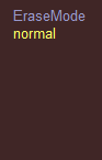
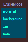
The popup pseudo object is highly customizable, but here is a typical example. On the left is the popup in its
closed state. Click on the current selection ("normal" in this example) and the popup will open as shown to the right.
Note that in its opened state the currently selected item is shown in bold. As you would expect, simply clicking on
the new selection you want, closes the popup with the new selection.
The following table describes the popup pseudo object properties that you may set and query, although
how to use these properties may not become clear until later when the commands are discussed:
Property
Name |
Property
Value |
| choices |
A cell array of strings specifying the choices given when the popup is selected.
If all the choices are numeric you can use a numeric array instead of the cell array.
For example [3 5 7.5] is equivalent to {'3' '5' '7.5'}.
|
| index |
An integer specifying the current choice (default = 1, i.e. the 1st element of the choices cell array).
After the popup is set to the specified index, the popup is closed if it had been open.
The callback is not normally called when the popup choice is set using the index parameter, however if you
specify the negative of the index desired, then the callback will be called after the index is set.
|
| callbk |
A callback to be executed when the popup value is changed.
If the callback is defined with a string, then:
Occurrences of '@IDX' will be replaced with the popup index.
Occurrences of '@STR' will be replaced with the popup string. |
position
or
pos |
[x y width height] for the opened popup in pixels or normalized units.
Two other options may be enabled by making the x or y value negative. Therefore these two lines are equivalent:
plt('pop','pos',[-.3 .5 .1 .2],...)
plt('pop','pos',[ .3 .5 .1 .2],'offset',0,...)
Likewise the following two lines are also equivalent:
plt('pop','pos',[.3 -.5 .1 .2],...)
plt('pop','pos',[.3 .5 .1 .2],'swap',0,...)
In both these examples the second line is preferred for its clarity. Refer to the descriptions
of the offset and swap parameters below. Note that you also can make both x and y negative
to enable both the offset and swap options.
If the position was specified previously you can use a scalar argument to modify just the height component
or a two element vector to modify just the width and height components. |
| offset |
y or [x y] which specifies the location of the closed popup relative to the opened popup.
x is set to 0.08 if it is not specified (where 0/1 represent horizontal position of the
left/right edges of the opened popup). The meaning of the y variable becomes clear by considering
the example where the choices cell array contained 4 elements. Then:
- y = 0: represents the vertical position of the bottom of the opened popup
- y = 0.5: represents the vertical position of choice{1} of the opened popup
- y = 1.5: represents the vertical position of choice{2} of the opened popup
- y = 2.5: represents the vertical position of choice{3} of the opened popup
- y = 3.5: represents the vertical position of choice{4} of the opened popup
- y = 4.0: represents the vertical position of the top of the opened popup
Note that negative values for x or y may be used to indicate that the closed popup position should be
to the left of or above the position of the opened popup.
If the offset parameter is not included, then the closed popup will be at the top of the opened popup,
i.e. at position [0.08 n] (where n is the number of popup choices).
To put the closed popup at the bottom of the opened popup simply include
'offset',0 in the parameter list.
|
| colorbk |
The background color used when the popup is open. (default = [0 .3 .4]); |
| colorfr |
The foreground color used when the popup is open. (default = [.1 1 .9]) |
| enable |
0=disable, 1=enable (default=1) |
| swap |
Normally a left-click on the pseudo popup control opens the popup to reveal the list of choices
while a right click merely advances to the next choice without opening the popup. Sometimes it is
useful to reverse the roles of the left and right-click - a mode I refer to as the "super-button"
mode. In fact if there is only a single choice, it behaves exactly like a uicontrol button in that
the only effect from clicking on it is that its callback is called. If there are two choices in
the choices cell array, it behaves similarly except that the button text toggles between the two
choices with every click. Usually if there are fewer than four choices, the super-button mode is
more convenient than the regular mode. The super-button mode is selected by including the swap
parameter in the argument list. Often you will want to make the super-button look at least somewhat
like a button by including a box around the super-button text. The color of this box is specified
by the swap parameter. For example swap,'blue' will draw a blue box around
the button text. Or instead of a Matlab color string, you can use an [r g b] color triple. Set the
parameter to zero to use the current foreground color (which defaults to [.1 1 .9]). If the parameter
is missing (which is only possible if the 'swap' argument is at the end) or if the parameter is
set to '' or [] or 'none'
then no box is drawn around the button text.
Sometimes it is useful to be able to toggle the super-button mode on or off interactively. This is
possible with the following quick procedure:
- First open the popup. (A left or a right click will do this, depending on which mode you are in.)
- Then use the mouse to move the figure window a very small amount (less than 15 pixels
in any direction).
- And finally close the popup by clicking on any of the choices in the drop down list.
The 15 pixel requirement makes it quite unlikely that this action is performed unintentionally,
especially since one rarely thinks of moving the figure while adjusting a control. The
text swap toggled will appear in the Matlab command window to assure
you that the operation worked as intended. |
| hide |
A list of objects to hide before opening the popup. When the popup is later closed, these
objects are shown again (unless they were hidden before the popup opened). The hide parameter is
used to remove the distraction of objects that overlap or are too close to the popup list.
If there is a zero in the list, before the list is used the zero will be replaced with the
handle (or handles) of the plot grid lines. (This is convenient because grid lines are the
most common object to overlap with opened popups.) Also setting the hide parameter to
'' or [] or not supplying a parameter
at all (only possible if the 'hide' argument is the last one) is equivalent to setting
the parameter to zero. |
| interp |
'none' or 'tex' (default='none') |
| label |
{'LabelString', offset, 'Property1',Value1,'Property2',Value2, ...}
A label for the popup will be created as a text object in the same axis that is used to display
the popup choices and will contain the string 'LabelString' (the first element of the cell array argument).
The 2nd element of the cell array is a complex number containing the offset for the label position in pixels
from the closed popup. (The real part is the x offset and the imaginary part is the y offset). For example
if the 2nd element of the cell array is -10+20i, then the label will be positioned 10 pixels to the left
and 20 pixels above the closed popup.
The remaining cell array elements (if any) must contain property/value pairs, and the properties must be valid
text object property names. The specified properties will be applied to the closed popup text string.
Specifying an offset of '' or [] is equivalent to
specifying the number 5 for this cell array element. (i.e. the default offset is 5 pixels to the left.)
Instead of specifying a cell array for the label argument, you may also specify a string. For example,
the argument 'LabelString' is equivalent to
{'LabelString',''}. Since the default offset is usually sufficient,
it turns out that this shorter form is used far more often than the cell array parameter. |
| labely |
This behaves just like the label parameter above except for the fact that the
default offset when it isn't specified is 16i (instead of 5 as is used by the
label parameter). This is the usual offset needed for placing the popup label
directly above the closed popup text. |
| ***** |
If a property name is given which isn't in the list above then the property is applied to
the popup text object itself. (It must be a valid text property.) The text color
('color') is usually set this way, however if that property is
not specified, the default color is [1 1 .4]. |
The following commands are used to create a popup pseudo object:
H = plt('pop',
'Poperty1',Value1,
'Poperty2',Value2,...)
| The property names allowed and the interpretation of the property values are shown in the table above.
You many use as many or as few properties as you need in whatever order you choose.
|
H = plt('pop',
[x y width height],
{'choice1', ... 'choiceN'},
'Poperty3',Value3,...)
| Both the 'position' and the 'choices' properties are required, so for conciseness you may omit those
property names if the property values appear first and in this order.
Property names other than these two may not be omitted.
|
H = plt('pop',
'pos',[x y width height],
'choices',{'choice1', ...},
'Poperty3',Value3,...)
| The above command is translated into this line before execution. Note that in any of these commands
you may use either pixel or normalized units. (You aren't required to included the 'units' property
since plt can figure out this property from the size of the numbers in the position vector.)
|
The above calls create a popup pseudo object and returns the handle of the text object that is
visible when the popup is closed. This handle (H) may be used to modify or query the popup pseudo
object parameters using the forms below:
plt('pop',H,
'Poperty1',Value1,
'Poperty2',Value2,...)
| If H is a scalar, the specified property values are applied to the popup pseudo object identified by handle H.
The property names are the same ones described in the table above.
If H is a vector then Property1 of H(k) is set to the kth row of Value1.
If Value1 doesn't have that many rows, the last row will be used. Only one
property is allowed for the case where H is a vector.
|
| plt('pop',H,'get','string') | returns the currently selected element of the choices cell array.
Equivalent to the shorter command: get(H,'string')
|
| plt('pop',H,'get','axis') | returns the handle of the axis used to display the opened popup.
|
| plt('pop',H,'get','choices') | returns the cell array of choices that was set via the 'choices' parameter
|
| plt('pop',H,'get','index') | returns the index number of the specified edit pseudo object (between 1 and the
length of the choices cell array).
For conciseness, this command may also be written without the last argument:
plt('pop',H,'get') or even without the last two arguments:
plt('pop',H)
|
| plt('pop',H,'get','callbk') | returns the function handle or string that was set via the 'callbk' parameter
|
| plt('pop',H,'get','offset') | returns the number or vector that was specified via the 'offset' parameter
|
| plt('pop',H,'get','colorfr') | returns the 3 element vector or color string that was specified via the 'colorfr' parameter
|
| plt('pop',H,'get','enable') | returns 0/1 if the pseudo object is disabled/enabled
|
| plt('pop',H,'get','hide') | returns the vector of handles that was set via the 'hide' parameter
|
| plt('pop',H,'get','interp') | returns the string that was set via the 'interp' parameter
|
| plt('pop',H,'get','label') | returns the label handle
|
| plt('pop',H,'get','swap') | returns true if the swap (super-button) mode is selected.
|
| plt('pop',H,'get','cell') | returns an 11 element cell array that is a concatenation of the
previous 11 get commands:
{axis choices index callbk offset colorfr enable hide interp label}. Note that this does not include
the first get command ('string') listed above. Also 'cell' in this call may be replaced by any string other than one
of the other 12 valid 'get' arguments.
|
| plt('pop',H,'open') | opens the popup revealing the popup choices.
|
Mouse behavior:
Left-clicking on the popup text object "opens" the popup. What this means is
that the popup string is replaced by a list of the popup choices (rendered using
colorfr/colorbk). The user then clicks on the desired choice which then becomes
the new text string. right-clicking on the popup text object changes the text
string to the next available choice. If the last choice is already selected,
then right-clicking will change the text string to the first available choice
(in the "choices" array). If you hold down the right mouse button, the
selection will continuously advance cyclically. You can alter the rate at which
the cycling proceeds by setting the figure application data
repeat property. The use of this property is more
completely explained above in the description of the edit pseudo object.
See both the gui2.m and the curves.m
example programs for ideas on how to use these
pseudo popup objects as well as the pseudo edit objects described above.
Also the pltsq.m and the wfall.m
examples show how to use this pseudo object to create a "super button"
used to start and stop a moving plot. |
|
slider(pseudo
slider
object)
|
|
When using a uicontrol slider to control a parameter in a GUI, besides the
slider object itself, one generally also wants an edit box to show the current
slider value as well as to allow data entry by typing a number. Also a label
is usually required to identify the data and two more labels indicating the minimum
and maximum allowed values are also desirable. The pseudo slider object combines
those five objects into one and is included in plt to make your GUIs easier to
design. The additional movement and quantization modes in particular often
greatly reduce the amount of code you need to make the control work as desired.
To create a slider pseudo object, use the command:
H = plt('slider',In1,In2,In3,In4,In5,In6,In7)
This creates a pseudo object which usually looks something like this:
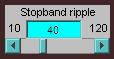
The five component uicontrols that are created for the pseudo object are identified as:
------------label----------
min ValueEditbox max
-----------slider----------
The variables used in the above slider initialization command are described below:
| H |
The return value is the pseudo slider's handle which is used to read and modify
the pseudo slider's properties. (See the get
and set commands below.) |
| In1 |
[x,y,width] in pixels or normalized units. Values less than one
are assumed to be normalized. Mixing units is ok although x & y must use the same units.
[x,y] are the coordinates of the lower left corner of the pseudo
slider label (which is also the upper left coordinate of the min value text). If
width is missing 120 is assumed.
When the position is specified with a 2 or 3 element as just described, the pseudo slider
will look similar to the object shown above which includes all 5 subcomponents. The second way to
specify the pseudo slider position is with a 4 element vector in the traditional Matlab format
(i.e. [xLeft,yBottom,Width,Height]). When using this form, the position
vector only specifies the position and size of the actual slider uicontrol. plt will calculate what
is hoped to be the optimal position and size of the label and edit box components. If the
Width value specified is larger than the Height
value, then the pseudo slider will end up looking similar to this:

Note that the min/max labels are not rendered when the position is specified this way which makes
it more compact. If the Width value is smaller than the Height value then the slider will be oriented
vertically with the label is placed at the top and the editbox placed at the bottom. (See the demo
programs bounce.m and pltmap.m for examples
of the use of both these forms. If the label and editbox are not wide enough for your taste you
can fix it by adding spaces to the left and right sides of the label, since plt uses the length of
the label string to determine the width of those two elements. Alternatively you may include a 5th
element to the position vector which specifies the width of both the label and the editbox. If
you are very picky, you can set In1 to be an eight element vector.
In that case, the first four elements specify the position of the slider component and the last
four elements specify the position of the label component (using the traditional Matlab positioning
style). The editbox component will then be set to be the same size as the label component and placed
on the opposite side of the slider from the label.
Finally there is one last method when complete flexibility is required where the
In1 argument is specified by a cell array. This cell array must have
5 elements which specify the positions of the Label, Slider, MinText, MaxText, and EditBox
components respectively. These positions must all be in either normalized or pixel units and
each component must be either a 4 element Matlab style position vector or an empty vector which
indicates that the associated element is to be invisible.
In1 is the only required parameter for this function. |
| In2 |
[value, smin, smax, emin, emax]
value is the initial value assigned to the slider.
smin/smax are the slider values at its leftmost/rightmost position.
emin/emax are the smallest/largest values allowed when entering numbers
into the edit box. If emin and emax are missing, 1e-99 and 1e99 are assumed.
If In2 is not supplied, [50 0 100] is assumed. |
| In3 |
Slider label. If you don't want a label, don't supply this parameter, or set
In3 to ''. |
| In4 |
Slider callback. This expression will be evaluated whenever the user moves the slider
control or enters a number in the edit box. Occurrences of '@VAL'
will be replaced with the current value. This parameter is optional, however you must include
it if you want to specify any of the three parameters shown below. If you need to supply
this parameter for that reason, but you don't need the callback, simply set
In4 to ''. |
| |
The following three parameters are optional. Although they have been identified as
In5,
In6, and
In7 in fact these three parameters (or any subset of them) may
be included in the argument list in any order you choose. (The data type is used to identify
which parameter is being supplied.)
|
| In5 |
This parameter controls how the slider moves when the slider left/right arrows are clicked
or when clicking in the space to the left or right of the slider button.
| In5 | Movement | Quantization |
| 1 |
Linear |
none |
| 2 |
Linear |
rounded to nearest integer |
| 3 |
Linear |
rounded to nearest power of two |
| [4 q] |
Linear |
rounded to nearest multiple of q |
| 5 |
Logarithmic |
none |
| [6 q] |
Linear |
rounded to nearest integer for slider arrows
and to nearest multiple of q for slider trough |
If In5 is not provided then 1 is assumed.
For modes 4 & 6, q defaults to 10 if not specified.
|
| In6 |
{fmin fval fmax}
fmin/fmax are formatting strings for the min/max labels and fval is the
formatting string for the edit box. These strings may contain c style
printf formatting codes or the W,V,w,v formats. (Type "help prin" for a
description of these formats).
You may use a space to delimit the formatting codes.
For example: '%4w %5.2f %2w'.
Or use a row or column cell array if you prefer:
{'%4w' '%5.2f' '%2w'}.
Since the w format is the most convenient format to use for this parameter,
for conciseness a single digit may be used as a shorthand for the w format.
So the example above may also be written as '4 %5.2f 2'
or as {'4' '%5.2f' '2'}.
Often it is sufficient to only specify the format for fval and accept the
defaults for fmin and fmax (which are '%2w'
and '%3w' respectively). We can
do this by simply specifying a single format code. For example
'%5.2f' is equivalent to
'2 %5.2f 3'.
If In6 is not provided, then '6' (or equivalently
'2 6 3') is assumed - i.e. the w format is used for all three elements. |
| In7 |
[LabelBG; EditBG; LabelFR; EditFR]
This is an array containing 3 columns and up to 4 rows. Columns
1/2/3 respectively represent the proportion (0 to 1.0) of red/green/blue
used in the control. The first two rows are the background colors for
the label and edit fields respectively. The last two rows are optional
and contain the label and edit field foreground colors. If the
foreground colors are not specified then black is assumed (i.e. [0 0 0]).
If In7 is not provided then [.75 .75 .75; 0 1 1] is assumed. |
For the commands below, H is the handle returned
from the above slider initialization command.
The get commands:
| plt('slider',H,'get','value') |
returns the pseudo slider's current value |
| plt('slider',H,'get') |
equivalent to the above |
| plt('slider',H) |
also equivalent to the above (the shortest and most cryptic method of getting the slider's value) |
| plt('slider',H,'get','visible') |
returns 1 if the slider is visible, 0 otherwise |
| plt('slider',H,'get','ena') |
returns 1 if the slider is enabled, 0 otherwise |
| plt('slider',H,'get','position') |
returns the slider position coordinates [x y width] in the same units as originally specified. |
| plt('slider',H,'get','pos') |
same as above |
| plt('slider',H,'get','obj') |
returns the slider object handles:
[ Label; Slider; MinText; MaxText; EditBox ] |
The set commands:
| plt('slider',H,'set',a) |
Sets the slider to value a.
Returns a possibly limited value. |
| plt('slider',H,'value',a) |
Equivalent to above. You may also use the extra parameter 'set' to add clarity as in
plt('slider',H,'set','value',a) if you prefer. In fact this
extra parameter is allowed (immediately after the slider handle) in all the remaining commands
shown in this table. |
| plt('slider',H,'val',a) |
Same as above except the slider callback is not executed |
| plt('slider',H,'position',a) |
Sets the slider position.
(See In1 in the slider initialization description above). |
| plt('slider',H,'pos',a) |
Same as above. |
| plt('slider',H,'minmax',a,b) |
a contains [smin,smax,emin,emax] (see In2 above)
b is a new slider value (optional)
Returns a possibly limited value. |
| plt('slider',H,'visON') |
Makes slider visible. |
| plt('slider',H,'visOFF) |
Makes the slider invisible. |
| plt('slider',H,'enaON') |
Enables the slider. |
| plt('slider',H,'enaOFF') |
Disables the slider |
| plt('slider',H,'label',a) |
Sets the label string to a. If a is empty, the label is made invisible. |
| plt('slider',H,'mode',a) |
Sets the slider movement mode. (See In5 above).
Returns a possibly limited value. |
|
|
image(pseudo
intensity
map
object)
|
|
Before getting much farther in this section, you should try running the
pltmap.m example program
so that you have a better context for the information that follows.
The Image pseudo object provides cursoring methods appropriate
for this object type and also includes several optional components including:
- A color bar which serves as a legend for the z-axis values as well as providing a method
of changing the colormap used to represent the z data.
- A slider (labeled 'edge') that allows you to control how wide a range around a midpoint
is used when determining the color used to represent each array element.
- A slider (labeled ''mid'') that allows you to control the center value of the range of values
used to determine the color for each array element.
- A checkbox that allows you to control the visibility of the axis gridlines.
- A 'view all' button, that when clicked on resets the axis limits associated with the image object
so that the entire image data set is visible. A secondary feature of this button is activated by
right-clicking on it instead. Each time you right-click on this button the axis limits are zoomed in to
expose only the middle 36% of the visible area. (This represents a 60% expansion of both the x and y axes.).
Initialization
h = plt('image',axI,x,y,z,opt);
The image object is created in an axis and figure that must be created beforehand using the plt pseudo object.
For example, suppose we create a figure with the command plt(x1,y1,x2,y2,'Subplot',[40 60]);
These creates two axes, the smaller one (40% of the height) below and the larger one on top. And suppose we
want to put the intensity map in the larger axis, then we would use
plt('image',2,x,y,z);.
I have set axI equal to 2 to indicate that the image should be inserted into the upper
plot (using the usual rules for the ordering of the axes). You wouldn't expect it matters what is in x2,y2 since
this trace is covered over by the image object, but in fact x2 should be set to the same array as the x vector
specified in the image initialization. This insures that the intensity map cursors operate correctly. (The data in
y2 on the other hand does not matter as long as it is the same length as x2).
opt is an optional cell array that specifies the image object options. This cell array
may contain any or all of the following strings in the following table. These strings are case insensitive, and
actually all characters except the first one are ignored. So for example 'view',
'ViewAll', and 'V' would all serve the same purpose.
| 'cbar' |
If this string is included the color bar image is created which serves as a color key
(i.e. for displaying the current color map). You can click on this color bar to cycle through
seven different color maps as follows:
- 0: rainbow
- 1: jet
- 2: sometric
- 3: seismic
- 4: gray
- 5: colorcube
- 6: lines
This entry is an exception to the rule that only the first character is significant, because you
may also include a digit between 0 and 6 as the last character of the string. This specifies which
color map to appear when the image object is initialized. For example 'cbar3',
'c3' or 'CbarSeismic3' all
would initialize the color map to "seismic". If the last digit of the string is not a digit then the
the rainbow color map is selected as the by default.
|
| 'edge' |
If this string is included the "edge" slider will appear which controls the range of the zData that is
mapped to the selected color map.
|
| 'mid' |
If this string is included, the "mid" slider will appear which controls the mid point of the zData range
that is mapped to the selected color map. The effect of adjusting this slider, as well as the "edge" slider
mentioned above is described in more detail in the description of pltmap.m
in the Programming examples section.
|
| 'grid' |
If this string is included, a "grid" checkbox will appear which allows you to turn the grid lines for the
image object on or off. This is an exception to the rule that the case is insensitive since 'Grid' and 'grid'
have slightly different meanings. They both create the checkbox, but the capitalized version initializes the
check box to 'on' (i.e. the grid lines are enabled) and the lower case version initializes the box to 'off'.
|
| 'view' |
If this string is included a "view all" button will appear which when left-clicked on will zoom the axis
so that the entire image data set is visible. As mentioned above, you may also zoom into the middle of the
visible region by right-clicking on this button. (The middle 60% of both the x and y axes will become visible.)
|
You may optionally include a 4 element position vector (in normalized coordinates) after any of these 5 options strings.
If the position vector is not included, then a default position is chosen for the item. For example:
opt = {'Cbar' [.5 .4 .02 .24] 'Grid' 'ViewAll' [.91 .75 .04 .02]};
When this option cell array is used for the image object initialization, a color bar, a grid checkbox, and a view all
button will be created, but the edge and mid sliders will not be since they are not included in the options list.
The color bar and view all button will be positioned at the coordinates given, whereas the grid checkbox will be
positioned at its default location since there is no position specified for it in the options list. You may use a
space or comma as a delimiter between option elements (i.e. row vector form as in the above), or you may use semicolons
if you prefer (i.e. column vector form).
The call that initializes the pseudo image object returns the image handle h
which you may then use in any of the image modification commands shown below. First we have the data
update commands which come in seven forms depending on which coordinates you want to update:
plt('image',h,'x',x);
plt('image',h,'y',y);
plt('image',h,'z',z);
plt('image',h,'xy',x,y);
plt('image',h,'xz',x,z);
plt('image',h,'yz',y,z);
plt('image',h,'xyz',x,y,z);
Then we have commands which can change the values of the mid and edge sliders (only allowed if they were created by
the image object initialization):
plt('image',h,'mid',Value);
plt('image',h,'edge',Value);
And finally we have commands to change the x and y limits:
plt('image',h,'xlim',[xLower xUpper]);
plt('image',h,'ylim',[yLower yUpper]);
For convenience you can combine any of the above image modification commands into a single command. For example
to change the y and z data values, adjust the edge slider and the y-axis limits you would use a command such as:
plt('image',h,'yz',y,z,'edge',1.5,'ylim',[0 5]);
|
|
ColorPick(pseudo
color select
object)
|
|
 Although
you will probably choose an attractive color scheme for your GUI
applications, the user's satisfaction with the application may be
greatly improved by allowing them to choose the colors used for the
major screen objects. By using the ColorPick pseudo object you allow the
user to efficiently choose the screen colors in a consistent way within and
among your applications. Also you will find that selecting colors using the
ColorPick figure is much easier than using the typical Windows style
palette which attempts to show all possible colors in a single palette.
I've found you need to see a fairly large area of your potential color choice
before you can decide if the color is suitable. It is not possible to accomplish
that using a single palette which is what makes it frustrating to use. By allowing
you to fix one of the colors, ColorPick presents an 11x11 palette of choices
for the remaining two colors which gives you plenty of area for each color block.
(If that is not enough, you can resize the ColorPick figure to be as large as you want.)
Even more important is that the instant you click on one of the 121 colors in the
current palette the larger patch above the palette AND the objects in the gui that you are
adjusting instantly change to the selected color. This instant feedback is really
necessary to remove the frustration that usually arises from the task. Scrolling through the
many possible palettes is also very quick. Just pick any slider and click on the
left/right arrows for a finely changing palette, or click in the trough area of
the slider for a more coarsely changing palette (which should be fine enough all
but the most picky color chooser). Although
you will probably choose an attractive color scheme for your GUI
applications, the user's satisfaction with the application may be
greatly improved by allowing them to choose the colors used for the
major screen objects. By using the ColorPick pseudo object you allow the
user to efficiently choose the screen colors in a consistent way within and
among your applications. Also you will find that selecting colors using the
ColorPick figure is much easier than using the typical Windows style
palette which attempts to show all possible colors in a single palette.
I've found you need to see a fairly large area of your potential color choice
before you can decide if the color is suitable. It is not possible to accomplish
that using a single palette which is what makes it frustrating to use. By allowing
you to fix one of the colors, ColorPick presents an 11x11 palette of choices
for the remaining two colors which gives you plenty of area for each color block.
(If that is not enough, you can resize the ColorPick figure to be as large as you want.)
Even more important is that the instant you click on one of the 121 colors in the
current palette the larger patch above the palette AND the objects in the gui that you are
adjusting instantly change to the selected color. This instant feedback is really
necessary to remove the frustration that usually arises from the task. Scrolling through the
many possible palettes is also very quick. Just pick any slider and click on the
left/right arrows for a finely changing palette, or click in the trough area of
the slider for a more coarsely changing palette (which should be fine enough all
but the most picky color chooser).
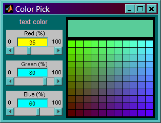
Any Matlab object that has either a callback property or a buttondownfunction
property may be used to bring up the ColorPick window shown here. Before I describe
how this is done from a programming perspective I will give a few more details about
how the user selects colors from this window.
The text above the sliders is generally used to identify the object or
objects that are to receive the color being selected. The three sliders
always indicate the RGB values of the currently selected color. In the example
shown at the left, the RGB values are
35%, 80%, and 60% respectively. In Matlab, this color would be represented
by the vector [0.35 0.8 0.6]. The large rectangular patch object
in the upper right corner always indicates the color that results when the
proportions are set to agree with the values of the three RGB sliders. One
of the sliders (the red one in this example) will always be shown with its
text value in yellow and is referred to as the "active slider". A slider
will become the active slider whenever you either type in a value into its
edit box or when you click on the left or right slider arrows. There are 3
ways to alter the currently selected color:
- You can simply select the desired color using the RGB sliders. Note that
with this method it is irrelevant which slider is identified as active.
- You can click on any one of the 121 small square patches that are arranged in an 11x11 grid.
The colors in this grid are entirely determined by the active slider. In this
example, since the active slider shows RED=35%, every color in the 11x11
color grid will have red = .35 with varying amounts of the other two colors.
So in this example, the colors of the the 4 corners of this grid starting at
the lower left and moving clockwise are:
[.35 0 0], [.35 1 0], [.35 1 1], and [.35 0 1]. and the square exactly in
the middle of this grid has the color [.35 .5 .5]. Clicking on any one of
these 121 patches will change the two inactive sliders to the values
associated with the patch that you clicked on. (The active slider will be
unchanged and will remain active). Also the large patch and all the objects in the
gui that are associated with this ColorPick object will change to show the new selected color.
- Clicking on the large patch will cause the
sliders to move to the "reset" values - i.e. the color that was in effect
when the ColorPick window was first opened. Note that this color never
changes for as long as the ColorPick window remains open. The reset values
may be changed to the values shown currently by the sliders by closing the
ColorPick window and re-opening it again.
Next I will describe how
the ColorPick object is created from the programmers viewpoint. I will call
the object that initiates the creation of the ColorPick figure window the
"main object". You must do the following two things to make a ColorPick
figure appear:
- You must assign an application data variable named 'm' to the main object with a
cell array of this form:
{'PROP1', H1, 'PROP2', H2, 'PROP3', H3, ... 'PROPn', Hn, 'label'}
When the user selects a new color using the
ColorPick figure, the 'PROP1' property of the object with handle H1 will be
set to the 3 element vector [R G B] where RGB are the values from the
ColorPick figure. If H1 is a row vector of handles, each of the represented
objects will be treated similarly. Then in sequence the objects in H2, H3
... Hn are treated in a like manner. If any of the 'PROPi' entries are
'str' or 'string', then the numerical 3 element color vector is converted to
an Ascii string before being assigned to that property. In place of any property
string, you may use a cell array of strings in which case ColorPick will assign
the user selected color to all the properties listed in the cell array of all
the handles listed in the following argument. Finally, the
last entry 'label' is optional, and if included will appear above the rgb
sliders and is used to identify what screen elements are being controlled.
- To the callback or buttondownfunction property (or both)
of the main object you must assign one of the following strings:
- 'plt ColorPick' This will cause the ColorPick
figure to be created when the callback or buttondownfunction is called
except for one special case - which is when the callback of an 'edit' style
uicontrol is called. The reason for this special case is that if you type
the desired colors directly into an edit box usually this indicates that you
didn't need the help of the ColorPick figure.
Note that in this special case, the properties listed in the 'm' application
data cell array are still modified as described above even though the
ColorPick figure is not created. Note that the ColorPick window will appear
when you right-click on such an edit box if the buttondownfunction of the
edit box has been similarly assigned.
- 'plt ColorPick ccf' This has the same effect as above
except that when the user changes a color with the ColorPick figure, in
addition to changing the properties in the 'm' cell array, the function
ccf is called. ccf stands for color change function and may be any string
corresponding to a function name and may include numerical arguments, such as
in 'plt ColorPick changeFunc(3,-1)'. In fact the function can have string
arguments as well although this is less convenient since you would need
two sets of quotes around each string argument. For example
'plt ColorPick changeFunc(''StringArg'')'. You should especially avoid color
change functions that required a string argument containing spaces
although if you really wanted to do that it would be possible with an
obscure looking callback such as
'plt(''ColorPick'',''changeFunc(''''A string argument'''')'')'
- 'plt ColorPick 0 0' is similar to case 1 above and plt ColorPick ccf 0' is similar to case 2 except that the special case relating to the edit box callback does not apply (i.e. the ColorPick window will be
created in every instance).
Only one detail remains to describe the operation of the ColorPick object,
and that has to do with how ColorPick determines the starting positions of
the RGB sliders when the window is first opened. This is a two step
process. First ColorPick must decide which object will be used to determine
the initial color. Once the object is chosen, ColorPick must decide which
property of this object to use. Here are the details of these two steps:
- Picking the object which will determine the initial color. Usually the
handle of the main object will be among one of the handles included in the
'm' application data cell array and in this case the main object itself is
used to determine the initial RGB slider positions. However sometimes this
is not the case. For example, in the demoplt.m program, we would like to
open the ColorPick window when we click on the text object "text color"
which serves as a label for the text color patch. However since this is just
a label, it is not entirely appropriate for the color of this text object to
change which means that it will not appear in the list of handles in the 'm'
cell array. So in this instance, ColorPick determines the initial color from
the object whose handle is the first element of H1 in the 'm' cell array.
(This is the only instance where the order of the handles in this array is
significant.)
- Picking the property of the selected object which determines the initial color.
- If the selected object is a uicontrol. If
the uicontrol is an edit box then its 'string' property is always used to
determine the initial color. If the string includes fewer than 3 numbers,
then extra zeros are added to the end of the vector. If the string includes
any numbers that are greater than one, then these numbers are clipped at one
and if any numbers are less than zero, then these numbers are clipped at
zero. If the uicontrol is not an edit box, then first the 'string' property
is examined to see if it represents a valid color vector (i.e. it must have
3 elements, all of which are between 0 and 1). If it is valid, than this
vector is used as the initial color. If it is not valid, the uicontrol
'backgroundcolor' property is used as the initial color.
- If the selected object is a text object, its 'string' property is used if this
string translates to a valid color vector. Otherwise the 'color' property of
the text object is used.
- If the selected object is a patch object, its 'facecolor' property is used as the
initial color.
- For all other object types, the 'color' property is used as the initial color.
|
|
HelpText(pseudo
text
object)
|
|
This pseudo object can be thought of as a super text object ... i.e. a collection
of text objects that can be created and deleted with a single command. The pseudo
object is created with either on of the following two commands:
plt('HelpText','set',v);
plt('HelpText','on',v);
where v
is a string or more commonly a cell array of strings and string properties. The HelpText
object is associated with the current figure window. Unlike the other pseudo objects, a
figure may contain only one HelpText object, which is why an object handle is not returned.
If you create a new HelpText object for a figure that already has one, the old one is simply
deleted before the new one is created.
The second form above ('on') is equivalent to the following two commands:
plt('HelpText','set',v);
plt('HelpText','on');
where the 'on' command is described below. Thus the two initialization forms are similar
except that when the first form is used the text will not become visible until the first
'on' command is issued, whereas with the second form, the text becomes visible immediately.
As mentioned in the
Labels and figure properties section you may also create a HelpText pseudo object
at the same time the plt pseudo object is created
by including 'HelpText',v in the parameter list of the call
to plt. (In fact, that is by far the most common way this pseudo object is created.)
Creating the HelpText that way is similar to the 'on' command above in that the help text
becomes visible right away (i.e. a separate HelpText 'on' command is not needed).
The structure of the v parameter is described in the table at the
bottom of this page, but first I'll list the commands used to control the HelpText object.
The functional form may be used but the command form is shown below since that is more
convenient when only string arguments are needed:
| plt HelpText on |
Although the pseudo object is created with the above 'set'
command, the individual text objects defined are not actually created until this
on command is given. Most often this command is used to
reenable the Help Text after it was turned off with the command shown below. |
plt HelpText
plt HelpText off |
Both of these forms are equivalent. They delete the text objects created by the above
on command. Often you will want the help text to disappear
once the user starts using the plot so it doesn't get in the way. One way to do this
is to include 'MoveCB','plt HelpText;' in the parameter
list when you are creating the plt pseudo object. This sets the move cursor callback
so that when you move the cursor or click on the plot, the help text will be removed. |
| plt('HelpText','get') |
This returns the v parameter that was used to create the HelpText object. There aren't many uses for this command, although one use would be to
copy a HelpText object from one figure to another.
|
| plt('HelpText','text') |
This returns a list of handles to text objects that were created after a helptext
'on' command has been executed. An empty list is returned
if the helptext object is currently off. Since Helptext is marked with a special user
value, an equivalent result is returned from the command
findobj(gcf,'user',355/113);
|
The easiest way to describe the structure of the v argument used
above is by a series of examples:
| 'abcdef' |
Using a single string for the v parameter doesn't give
the resulting HelpText object much utility beyond the underlying text object it creates
but this is still sometimes useful because it is so easy to create along with the plt pseudo object. |
| {'abcdef' -.1+.5i} |
At a minimum you will most likely at least include a location for the text object. The location is
specified by a complex number with the real part giving the horizontal position and the imaginary
part giving the vertical position. In this example the horizontal position is to the left of the
main axis (by 10% of the plot) and the vertical position is at the middle of the main plot.
If the location is not specified (as in the example above) the position used is .03+.96i |
{'abc' 'def' 'line3' .5+.96i
'color' 'white' 'fontsize' 20} |
Each text string may be as many lines as you want (3 lines in this example). After the position
element you may specify as many property value pairs as you need. Only text properties are
allowed. If the text color is not specified, the default color [1 .6 0] is used. The font size will
default to 12 if not specified. Note that for this form (as well as the following one below), the
position value (complex) is required. This helptext argument must be a row cell array. (A column
cell array will not produce the expected result.) |
| {'ab' 'cd' .5+.9i 'color' [1 0 0] 2i 'line3' .1+.1i 2i 'line4' .9+.9i 'fontweight' 'bold'} |
With the full generality, you may define as many strings as you want, with each of these
strings being in different locations with different string properties. This example creates
three strings, the first of which is two lines. The "2i" (which occurs twice) in this example
is a separator that indicates a new string is about to be defined. Actually any
complex number will serve the same purpose, but my habit is to always use "2i" for this
separator to make it easy to recognize.
In this example, the first two help lines ('ab' & 'cd') will be red because the text is followed
by the color specifier [1 0 0]. However the next two lines ('line3' & 'line4') have no color
specifier, so they will be in the default color ([1 .6 0]). However if you change the
2i that appears just before 'line3'
to a -2i then line3 will also be red. This is because a delimiter
with a negative imaginary component indicates that you want all the properties specified for
the previous helptext line to apply to the current one as well. If you changed the next
2i to a -2i as well, then all the help
lines defined will be red. If the same property is included both after the text string and
in the carry over property list (enabled by the negative imaginary component) then the
property value after the text string takes priority.
|
Many of the demo programs (including curves, editz, gauss, gui2, julia, pltquiv, subplt, tasplt, trigplt, and wfalltst) create a HelpText
pseudo object, so you can refer to these programs to see practical examples of the use of the HelpText pseudo object.
|
|